Follow the discussion on Hacker News
Get this IJulia notebook on Github
The colors of chemistry
This notebook documents my exploration of color theory and its applications to photochemistry. It also shows off the functionality of several Julia packages: Color.jl for color theory and colorimetry, SIUnits.jl for unitful computations, and Gadfly.jl for graph plotting.
using Color, Gadfly, SIUnits, SIUnits.ShortUnits
Color vision and the visible spectrum
Physically speaking, light is radiation in the form of electromagnetic waves, and can therefore be quantified by certain characteristics such as wavelength and amplitude. Color theory studies how such characteristics get translated into a sensory perception, of color.
The human eye supports two types of vision: photoptic vision occurs under bright light, and scotopic vision occurs under dim light. These two modes come from using different types of vision cells, namely cones and rods respectively. Only cones sense color, and are sensitive to light with wavelengths in the range of 350-800 nm. The actual range can vary from person to person.
Color theory focuses mainly on photoptic vision in the 380-780 nm region. Computations for color theory are provided by functions in the Julia package Color.jl. For example, cie_color_match calculates the perceived color produced by monochromatic light, i.e. light waves of a single, pure wavelength.
#Define custom type to plot nicely with rainbow-like swatch
type ColorVector{T<:ColorValue} <: AbstractVector{T}
    C :: Vector{T}
end
import Base: size, writemime
size(C::ColorVector) = size(C.C)

function writemime(io::IO, ::MIME"image/svg+xml", cs::ColorVector)
    n = length(cs.C)
    width=0.5
    pad=0
    write(io, """
        <?xml version="1.0" encoding="UTF-8"?>
        <!DOCTYPE svg PUBLIC "-//W3C//DTD SVG 1.1//EN"
         "http://www.w3.org/Graphics/SVG/1.1/DTD/svg11.dtd">
        <svg xmlns="http://www.w3.org/2000/svg" version="1.1"
             width="$(n*width)mm" height="25mm"
             shape-rendering="crispEdges">
        """)
    for (i, c) in enumerate(cs.C)
        write(io,
            """
            <rect x="$((i-1)*width)mm" width="$(width - pad)mm" height="100%"
                  fill="#$(hex(c))" stroke="none" />
            """)
    end
    write(io, "</svg>")
end

rainbow = ColorVector([cie_color_match(λ) for λ=380:1.5:780])
Raw light power and the XYZ color space
The modern foundations of color theory can be traced back to the CIE 1931 color space model. Building upon centuries of empirical evidence that three coordinates are sufficient to quantify perceived colors, the CIE model defines three basis functions $\overline{x}(\lambda)$, $\overline{y}(\lambda)$ and $\overline{z}(\lambda)$ over (most of) the visible wavelength range 380nm $\le\lambda\le$780 nm.
These basis functions define a linear vector space known as the XYZ color space. An arbitrary function $f(\lambda)$ has a three-dimensional projection as a vector in this vector space, with components known as tristimulus values that are given by the projections
$$ X = \int f(\lambda) \overline{x}(\lambda) d\lambda $$ $$ Y = \int f(\lambda) \overline{y}(\lambda) d\lambda $$ $$ Z = \int f(\lambda) \overline{z}(\lambda) d\lambda $$
The CIE standard defines the basis functions in discrete tabular form; the raw data for $\overline{x}(\lambda)$, $\overline{y}(\lambda)$ and $\overline{z}(\lambda)$ are available in Color.cie_color_match_table[:,i] for i=1:3 respectively.
#Creates a plot layer for each color transfer function (ctf)
ctf_layer(i)=layer(Geom.line,
  x=380:780, y=Color.cie_color_match_table[:,i],
  color=fill(string('x'+i-1, '̄'), 401), #Generate name of ctf
)

#Plot the X, Y and Z ctfs
plot(Guide.XLabel("λ (nm)"), Guide.YLabel("Sensitivity"),
  Guide.colorkey("ctf"),
  #color each ctf by wavelength of peak sensitivity
  Scale.discrete_color_manual(
    map(cie_color_match, 379.+
    [indmax(Color.cie_color_match_table[:,i]) for i=1:3])...),
  [ctf_layer(i) for i=1:3]...,
)
Computing white
As a sanity check, I wanted to make sure that projecting a flat power spectrum into the XYZ space produced a white color. This is white in the purely technical sense, of having the same intensity of light at every wavelength.
To do this, we'll have to imbue the XYZ color space with vector space operations; in particular, we want to add and scale vectors. It follows by the definition of the XYZ color space that the usual notions of these operations apply (the color space has no curvature). These operations are not currently in Color.jl, but Julia makes it very easy to extend:
#The XYZ color space is a linear vector space
#So these operations make sense!
+(a::XYZ, b::XYZ) = XYZ(a.x+b.x,a.y+b.y,a.z+b.z)
*(a::Real,c::XYZ) = XYZ(a*c.x,  a*c.y,  a*c.z)
With these two operations defined, we can now proceed to compute the projections, which are convolutions against the basis functions.
@show mapreduce(cie_color_match, +, 380:780)
Ok, this looks like white. However, there's some built-in assumption on the normalization in Color.jl which I haven't figured out yet, which means that any XYZ(X,Y,Z) for sufficiently positive (X,Y,Z) will render as white.
The easy solution to this is to convert to the xyY color space, where $x$ and $y$ are (normalized) chromaticity coordinates (such that $x+y+z=1$) and $Y$ is the luminosity. Here's what the monochromatic rainbow looks like in this coordinate system:
rainbowxyY = map(λ->convert(xyY, cie_color_match(λ)), 380:780)
plot(Geom.point, Theme(key_position=:none),
    x=[c.x for c in rainbowxyY], y=[c.y for c in rainbowxyY],
    color=[1:length(rainbowxyY)],
    Scale.discrete_color_manual(rainbow.C...))
It is easy to normalize the perceptual color in the xyY coordinate system.
#Convert XYZ to normalized xyY (with luminosity Y=1.0)
function normalize0(c::XYZ)
    d=convert(xyY, c)
    xyY(d.x, d.y, 1.0)
end

#Convolution with flat power spectrum
mapreduce(cie_color_match, +, 380:780) |> normalize0
Oops, this isn't white. What's going on?
Turns out that this is a white point issue. The definition I wanted turns out to be the E white point (Color.WP_E), whereas the CIE standard uses a different default white point (Color.WP_DEFAULT), which is the D65 white point (Color.WP_D65, the 'noon daylight' standard used by most displays). Conveniently, Color.jl provides Color.whitebalance to correct for the difference in white points. So let's try this again.
#Convert XYZ to normalized xyY with white balancing
function normalize(c::XYZ; docorrect::Bool=true)
    d = convert(xyY, docorrect ?
      Color.whitebalance(c, Color.WP_E, Color.WP_DEFAULT) : c)
    xyY(d.x, d.y, 1.0)
end

#Convolution with flat power spectrum
mapreduce(cie_color_match, +, 380:780) |> normalize
Ok, this looks white now. We're ready to start visualizing some physical data!
Blackbody radiation
Perhaps the easiest physically relevant power spectrum to look at is that of blackbody radiation, which is described by Planck's law:
$$ B_\lambda (T) = \frac{2hc^2}{\lambda^5} \frac{1}{\left(\exp\left(\frac{hc}{kT}\right) - 1\right)} $$
The function definition below makes use of the SIUnits.jl package for defining unitful physical quantities.
#Power spectrum for blackbody using Planck's law
const hc_k  = 0.0143877696*K*m
const twohc²= 1.19104287e-16*Watt*m^2
planck{S1<:Real, S2<:Real}(λ::quantity(S1,Meter); T::quantity(S2,Kelvin)=5778.0K) =
    λ≤0m ? zero(λ)*Watt*m^-4 : twohc²*λ^-5.0/(exp(hc_k/(λ*T))-1)

Trange = 1000K:1000K:9000K
plot([λ->planck(λ*nm,T=T)*(1e-9m)^3/W for T in Trange], 0, 2000,
  Guide.xlabel("λ (nm)"),
  Guide.ylabel("spectral radiance, B (W·sr⁻¹·nm⁻³)"),
  color=[string(T) for T in Trange],
)
Let's look at the computed colors for blackbodies at various temperatures. The code below defines a new conversion function from temperature to an xyY color. (Note: For some reason, I got better results by disabling color correction in normalize. I'm not sure why.)
import Base.convert
convert{S<:Real}(::Type{xyY}, T::quantity(S, K)) =
  mapreduce(λ->planck(λ*nm,T=T)*m^3/Watt*cie_color_match(λ), +, 380:780) |>
  normalize0

blackbodies = xyY[convert(xyY, T) for T in 30K:30K:10000K]
ColorVector(blackbodies)
T☉=5778K #Temperature of the sun
@show convert(xyY, T☉)
To check the computed color, we can compare our computed color against what is called the Planckian locus, which is the trajectory in the chromaticity space $(x, y)$. There are known approximations using cubic splines as a function of the reciprocal temperature $1/T$.
Color.jl also provides a colordiff function which quantifies the distance between two colors using the CIEDE2000 color-difference formula (pdf). (I'm not sure what the units are though.)
#Use cubic spline formula from Wikipedia
function planckian_locus{S<:Real}(T::quantity(S, K))
    T=T/K#Strip out the unit
    x = 1667<=T<=4000 ? -0.2661239e9/T^3-0.2343580e6/T^2+0.8776956e3/T+0.179910 :
        4000<=T<=25000? -3.0258469e9/T^3+2.1070379e6/T^2+0.2226347e3/T+0.230390 :
        error("Temperature T=$T exceeds allowed limits of 1667<=T<=25000")
    y = 1667<=T<=2222 ? -1.1063814x^3-1.34811020x^2+2.18555832x-0.20219683 :
        2222<=T<=4000 ? -0.9549476x^3-1.37418593x^2+2.09137015x-0.16748867 :
        4000<=T<=25000?  3.0817580x^3-5.87338670x^2+3.75112997x-0.37001483 :
        error("Temperature T=$T exceeds allowed limits of 1667<=T<=25000")
    xyY(x, y, 1.0)
end

sun_approx = planckian_locus(T☉)
sun        = convert(xyY, T☉)

display([sun_approx, sun])
println(sun_approx)
println(sun)
println(colordiff(sun_approx, sun))
As a final check, overlay the approximate Planckian locus with the computed one from the blackbody spectrum. Close enough, maybe?
locus = map(T->planckian_locus(T*K), 1667:30:25000)

#XXX plotting issue https://github.com/dcjones/Gadfly.jl/issues/317
plot(Guide.xlabel("x"), Guide.ylabel("y"),
  layer(Geom.line, x=[c.x for c in blackbodies], y=[c.y for c in blackbodies], Theme(default_color=color("red"))),
  layer(Geom.point, x=repmat([sun.x], 2), y=repmat([sun.y], 2), Theme(default_color=color("red"))),
  layer(Geom.label, x=[sun.x], y=[sun.y], label=["☉"]),

  layer(Geom.line, x=[c.x for c in locus], y=[c.y for c in locus], Theme(default_color=color("purple"))),
  layer(Geom.point, x=repmat([sun_approx.x], 2), y=repmat([sun_approx.y], 2), Theme(default_color=color("purple"))),
  layer(Geom.label, x=[sun_approx.x], y=[sun_approx.y], label=["☉ (approx)"]),
)
The chemistry of color
With all this machinery in place to process power spectra, we can start to work with some really interesting data from the field of photochemistry. Chemists have measured the spectra of light absorbed and emitted from a large variety of molecules. From this data, it is possible to compute the perceived color of a given molecule.
The spectral data come in several formats which require further processing. The light absorption properties of molecules can be reported in terms of absorbance, optical density, optical cross section, molar extinction coefficient, complex refractive index, etc., which are essentially the logarithm of a normalized transmittance, the ratio of light intensities going through a sample vs. the intensity going in.
abstract Spectrum{T<:Real}

immutable AbsorbanceSpectrum{T<:Real} <: Spectrum{T}
    λ :: Vector{T}
    ϵ :: Vector{T} #Extinction coefficent, absorption cross-section or the like
end
AbsorbanceSpectrum(λ::Vector, ϵ::Vector) = AbsorbanceSpectrum(float(λ), float(ϵ))

immutable TransmissionSpectrum{T<:Real} <: Spectrum{T}
    λ :: Vector{T}
    T :: Vector{T} #Transmission coefficent
end

import Base.show
function show(S::AbsorbanceSpectrum)
    plot(Geom.line, Guide.xlabel("λ (nm)"), Guide.ylabel("Absorbance"),
      x=S.λ, y=S.ϵ)
end

function show(S::TransmissionSpectrum)
    plot(Geom.line, Guide.xlabel("λ (nm)"), Guide.ylabel("Transmittance"),
      x=S.λ, y=S.T)
end

function show(Ss::Vector{TransmissionSpectrum})
    plot(Guide.xlabel("λ (nm)"), Guide.ylabel("Transmittance"),
    [layer(Geom.line, x=S.λ, y=S.T) for S in Ss]...)
end
We can reconstruct the transmittance spectrum from the corresponding absorbance spectrum using the Beer-Lambert law:
$$T = {10}^{-c l \epsilon} = e^{-\sigma l N}$$
where $T$ is the transmittance, $\epsilon$ is the (decadic) molar extinction coefficent, $c$ is the molar concentration of the sample, $l$ is the optical path length, the distance light travels in the sample, $\sigma$ is the optical cross-section, and $N$ is the number concentration of the sample.
convert(::Type{TransmissionSpectrum}, S::AbsorbanceSpectrum; cl::Real=0.0001) =
TransmissionSpectrum(S.λ, exp10(-S.ϵ*cl)) #Beer-Lambert Law
The transmission spectrum is a function of light intensity over wavelength, and can therefore be projected directly into the XYZ color space as described in the previous section. (In the code snippet below, I've also included some heuristics to cover possible missing data in the transmission spectrum.)
function convert(::Type{xyY}, S::TransmissionSpectrum)
    #Calculate convolution of spectrum with XYZ color transfer functions
    color = reduce(+, [0.0; map(abs, diff(S.λ))].*S.T.*map(cie_color_match, S.λ))
    #Add in any missing parts of the spectrum (extrapolate spectrum from its endpoints)
    if (lolim=floor(minimum(S.λ))) > 380
        color += S.T[1]*reduce(+, map(cie_color_match, 380:lolim))
    end
    if (hilim=ceil(maximum(S.λ))) < 780
        color += S.T[end]*reduce(+, map(cie_color_match, hilim:780))
    end
    convert(xyY, color)
end

convert(::Type{xyY}, S::AbsorbanceSpectrum) = convert(xyY, convert(TransmissionSpectrum, S))
However, this reconstruction requires information about the concentration and thickness of the sample, which is normalized out in most reported data. What we can do here is to explore how the perceived color depends on the concentration. Here I've chosen to vary the concentration factor $cl=\sigma N$ by sweeping over the maximal transmittance $T_{max}$ in the visible spectrum:
$$cl = - \frac{log_{10}(T_{max})}{\epsilon}$$
and the computed color can be plotted in the $xy$ chromaticity plane as a function of the concentration factor.
#Compute a series of transmission spectra scaled to a desired maximum transmission
function calc_transmission(A::AbsorbanceSpectrum; maxTs=1.0:-0.0025:0.0)
    colors = xyY[]
    spectra = TransmissionSpectrum[]
    for maxT in maxTs
        scalefactor = -log10(maxT)/minimum(A.ϵ[A.ϵ.>0])
        T = convert(TransmissionSpectrum, A, cl=scalefactor)
        push!(spectra, T)
        push!(colors, convert(xyY, T))
    end
    colors, spectra
end

#Plot trajectory in chromaticity plane
plot_xy(C::AbstractVector{xyY}) = plot(x=[c.x for c in C],
    y=[c.y for c in C], color=[1:length(C)],
    Scale.discrete_color_manual(C...),
    Geom.point, Theme(key_position=:none))
Finally, here are some short routines for parsing spectral data.
function parse_jcampdx(filename)
    #This supports only the uncompressed JCAMP-DX file format
    #which is essentially CSV with a header
    rawspectrum=readcsv(filename, skipstart=20)
    #The columns are wavelength (nm) and log10 of molar extinction coefficient (M-1 cm-1)
    AbsorbanceSpectrum(rawspectrum[:,1], exp10(rawspectrum[:,2]))
end

function parse_photochemcad(filename)
    rawspectrum=readdlm(filename, '\t')
    rawspectrum=reshape(rawspectrum, (length(rawspectrum)÷2,2))

    #The columns are wavelength (nm) and molar extinction coefficient (M-1 cm-1)
    AbsorbanceSpectrum(rawspectrum[:,1],
      max(rawspectrum[:,2], 0.0)) #truncate negative extinctions
end
We are finally ready to start computing colors of molecules! The examples given below reflect (so to speak) a broad spectrum (ha) of molecular species, whose data are available online in several different formats.
I've also included some images of the compounds in question to compare the computed color swatches with pictures of the actual solutions or samples. Again, the color swatches show the entire gamut of colors possible from the given spectra, so each a picture should match a color in the range. (There's also a question about the white balance in each reference picture, which is somewhat of a wildcard.)
Titanium (III) aqua ion
filename=download("http://wwwchem.uwimona.edu.jm/spectra/ti3aq.jdx")
rawspectrum=readdlm(filename, skipstart=30)
#The columns are wavelength (nm) and absorbance (arbitrary units)
A=AbsorbanceSpectrum(rawspectrum[:,1], rawspectrum[:,2])

function showcolors(A::AbsorbanceSpectrum)
    colors, Ts=calc_transmission(A)
    display(show(A))
    display(show(Ts[1:20:end]))
    display(plot_xy(colors))
    display(ColorVector(colors))
end
showcolors(A)
Here is a picture of titanium (III) chloride solution from Wikipedia.
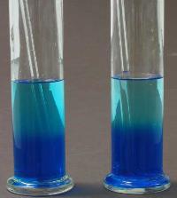
Copper (II) aqua ion
filename=download("http://wwwchem.uwimona.edu.jm/spectra/cu2aq.jdx")
rawspectrum=readdlm(filename, skipstart=30)
#The columns are wavelength (nm) and absorbance (arbitrary units)
A=AbsorbanceSpectrum(rawspectrum[:,1], rawspectrum[:,2])
showcolors(A)
I found a particularly nice picture showing the diffusion of copper sulfate through an aqueous solution, showing a color gradient which corresponds very neatly with the gradient shown in the gamut!
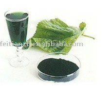
Copper(II) chlorophyllin
This chlorophyll derivative is used as an edible dye (food additive E141) to give food the color of fresh leaves. So one would expect this to be a nice shade of green.
filename=download("http://wwwchem.uwimona.edu.jm/spectra/e141.jdx")
rawspectrum=readdlm(filename, skipstart=30)
#The columns are wavelength (nm) and molar extinction coefficient (M-1 cm-1)

A=AbsorbanceSpectrum(rawspectrum[:,1], rawspectrum[:,2])
showcolors(A)
Azobenzene
Azobenzene is an azo compound which demonstrates a particular chemical reaction known as photoisomerization.
#Download UV-vis spectrum from NIST Chemistry Webbook
jcampid = "C103333"    #azobenzene

A=parse_jcampdx(download("http://webbook.nist.gov/cgi/cbook.cgi?JCAMP=$(jcampid)&Index=0&Type=UVVis"))
showcolors(A)
Here is a picture of a thin film made from azobenzene.

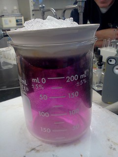
Dichromate [Cr$_2$O$_7$]$^{2-}$
filename=download("http://wwwchem.uwimona.edu.jm/spectra/cr2o7.jdx")
rawspectrum=readdlm(filename, skipstart=30)
#The columns are wavelength (nm) and absorbance (arbitrary units)
A=AbsorbanceSpectrum(rawspectrum[:,1], rawspectrum[:,2])
showcolors(A)

Pentacene
#Download UV-vis spectrum from NIST Chemistry Webbook
#jcampid = "C196203"    #9,10-Dibromoanthracene
jcampid = "C135488"     #pentacene

A=parse_jcampdx(download("http://webbook.nist.gov/cgi/cbook.cgi?JCAMP=$(jcampid)&Index=0&Type=UVVis"))
showcolors(A)

Rhodamine B
#A=parse_photochemcad(download("http://omlc.ogi.edu/spectra/PhotochemCAD/data/009-abs.txt"))

#Smooth out A with a simple moving average
function sma{T}(A::AbstractVector{T}, n=8)
    B=copy(A)
    avg=sum(A[1:n])/n
    for i=n+1:length(A)
        avg += (A[i] - A[i-n])/n
        B[i] = avg
    end
    B
end
B=copy(A.ϵ)
B[A.λ .> 600] = 0 #Zero out some noise
B=sma(B)
showcolors(AbsorbanceSpectrum(A.λ, B))

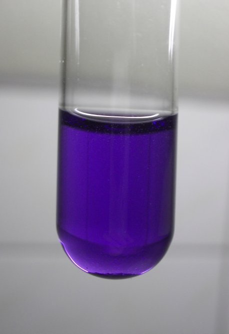
Iodine
#Data source:
#The MPI-Mainz UV/VIS Spectral Atlas
#of Gaseous Molecules of Atmospheric Interest
filename=download("http://joseba.mpch-mainz.mpg.de/spectral_atlas_data/cross_sections/Halogens+mixed%20halogens/I2_Tellinghuisen(2011)_308K_390-900nm.txt")
S=readdlm(filename, skipstart=2)
A=AbsorbanceSpectrum(S[:,1], S[:,2])
showcolors(A)
Here is an image of sublimed elemental iodine, showing off its famous purple color.
(It's interesting to see how to perceived colors change as a function of concentration - it's common knowledge in photochemistry that perceptual colors may change in this way, and that looking for new structure in the spectrum is the only sure way to detect further chemical reactions which may cause colors to change even more drastically.)